Introduction to ERT and Ensemble based methods

The reservoir model for a green field is based on a range of subsurface input including seismic data, a geological concept, well logs and fluid samples. All of this data is uncertain, and it is quite obvious that the resulting reservoir model is quite uncertain. Although uncertain - reservoir models are still the only tool we have when we make reservoir management decisions for the future.

Since reservoir models are very important for future predictions there is much focus on reducing the uncertainty in the models. When the field has been in production for some time one can use true data assembled from the producing field to update the model. This process is commonly called history matching in the petroleum industry, in this manual we will use the term model updating. Before the model updating process can start you will need:

1. A reservoir model which has been parameterized with a parameter set \(\{\lambda\}\).
2. Observation data from the producing field \(d\).

Then the the actual model updating goes like this:

1. Simulate the behaviour of the field and assemble simulated data \(s\).
2. Compare the simulated simulated data \(s\) with the observed data \(d\).
3. Based on the misfit between \(s\) and \(d\) updated parameters \(\{\lambda'\}\) are calculated.

Model updating falls into the general category of inverse problems - i.e. we know the results and want to determine the input parameters which reproduce these results. In statistical literature the the process is often called conditioning.

It is very important to remember that the sole reason for doing model updating is to be able to make better predictions for the future, the history has happened already anyway!

Embrace the uncertainty

The main purpose of the model updating process is to reduce the uncertainty in the description of the reservoir, however it is important to remember that the goal is not to get rid of all the uncertainty and find one true answer. There are two reasons for this:

1. The data used when conditioning the model is also uncertain. E.g. measurements of e.g. water cut and GOR is limited by the precision in the measurement apparatus and also the allocation procedures. For example for 4D seismic the uncertainty is large.
2. The model updating process will take place in the abstract space spanned by the parameters \(\{\lambda\}\) - unless you are working on a synthetic example the real reservoir is certainly not in this space.

So the goal is to update the parameters \(\{\lambda\}\) so that the simulations agree with the observations on average, with a variability which is of the same order of magnitude as the uncertainty in the observations. The assumption is then that if this model is used for predictions it will be unbiased and give a realistic estimate of the future uncertainty. This illustrated in figure ensemble.

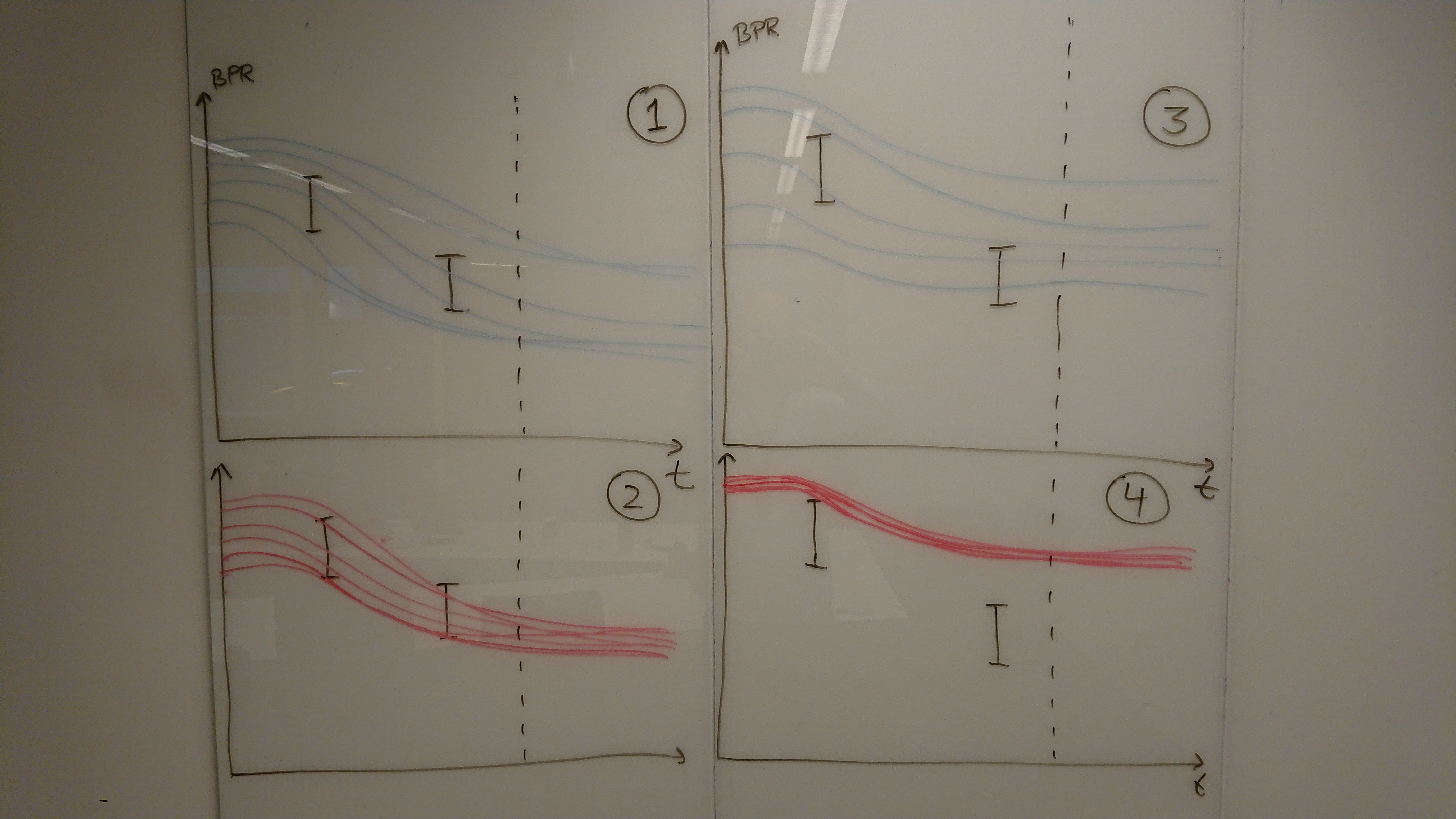
Ensemble plots before and after model updating, for one succesfull updating and one updating which has gone wrong.

All the plots show simulations pressure in a cell as a function of time, with measurements. Plots (1) and (3) show simulations before the model updating (i.e. the prior) and plots (2) and (4) show the plots after the update process (the posterior). The dashed vertical line is meant to illustrate the change from history to prediction.

The left case with plots (1) and (2) is a succesfull history matching project. The simulations from the posterior distribution are centered around the observed values and the spread - i.e. uncertainty - is of the same order of magnitude as the observation uncertainty. From this case we can reasonably expect that predictions will be unbiased with an reasonable estimate of the uncertainty.

For the right hand case shown in plots (3) and (4) the model updating has not been successfull and more work is required. Looking at the posterior solution we see that the simulations are not centered around the observed values, when the observed values from the historical period are not correctly reproduced there is no reason to assume that the predictions will be correct either. Furthermore we see that the uncertainty in the posterior case (4) is much smaller than the uncertainty in the observations - this does not make sense; although our goal is to reduce the uncertainty it should not be reduced significantly beyond the uncertainty in the observations. The predictions from (4) will most probably be biased and greatly underestimate the future uncertainty [1].

[1]	: It should be emphasized that plots (3) and (4) show one simulated quantity from an assumed larger set of observations, in general there has been a different set of observations which has induced these large and unwanted updates.

Ensemble Kalman Filter - EnKF

The ERT application was originally devised created to do model updating of reservoir models with the EnKF algorithm. The experience from real world models was that EnKF was not very suitable for reservoir applications, and ERT has since changed to the Ensemble Smoother (ES) which can be said to be a simplified version of the EnKF. But the characteristics of the EnKF algorithm still influence many of the design decisions in ERT, it therefor makes sense to give a short introduction to the Kalman Filter and EnKF.

The Kalman Filter

The Kalman FIlter originates in electronics the 60’s. The Kalman filter is widely used, especially in applications where positioning is the goal - e.g. the GPS system. The typical ingredients where the Kalman filter can be interesting to try include:

1. We want to determine the final state of the system - this can typically the the position.
2. The starting position is uncertain.
3. There is an equation of motion - or forward model - which describes how the system evolves in time.
4. At fixed point in time we can observe the system, these observations are uncertain.

As a very simple application of the Kalman Filter, assume that we wish to estimate the position of a boat as \(x(t)\); we know where the boat starts (initial condition), we have an equation for how the boat moves with time and at selected points in time \(t_k\) we get measurements of the position. The quantities of interest are:

\(x_k\)

The estimated position at time \(t_k\).

\(\sigma_k\)

The uncertainty in the position at time \(t_k\).

\(x_k^{\ast}\)

The estimated/forecasted position at time \(t_k\) - this is the position estimated from \(x_{k-1}\) and \(f(x,t)\), but before the observed data \(d_k\) is taken into account.

\(d_k\) The observed values which are used in the updating process, the

\(d_k\) values are measured with a process external to the model updating.

\(\sigma_d\) The uncertainty in the measurement \(d_k\) - a reliable

estimate of this uncertainty is essential for the algorithm to place “correct” weight on the measured values.

\(f(x,t)\)

The equation of motion - forward model - which propagates

\(x_{k-1} \to x_k^{\ast}\)

The purpose of the Kalman Filter is to determine an updated \(x_k\) from \(x_{k-1}\) and \(d_k\). The updated \(x_k\) is the value which minimizes the variance \(\sigma_k\). The equations for updated position and uncertainty are:

\[x_k = x_k^{\ast}\frac{\sigma_d^2}{\sigma_k^2 + \sigma_d^2} + x_d \frac{\sigma_k^2}{\sigma_k^2 + \sigma_d^2}\]

\[\sigma_k^2 = \sigma_k^i{2\ast}\left(1 - \frac{\sigma_k^{2\ast}}{\sigma_d^2 + \sigma_k^{2\ast}}\right)\]

Looking at the equation for the position update we see that the analyzed position \(x_k\) is a weighted sum over the forecasted positon \(x_k^{\ast}\) and measured position \(d_k\) - where the weighting depends on the relative weight of the uncertainties \(\sigma_k^{\ast}\) and \(\sigma_d\). For the updated uncertainty the key take away message is that the updated uncertainty will always be smaller than the forecasted uncertainty: \(\sigma_k < \sigma_k^{\ast}\).

Using an ensemble to estimate the uncertainty: EnKF

Ensemble Smoother - ES